The mlts package allows fitting multilevel manifest or
latent time series models and dynamic structural equation models (DSEM),
as described in Asparouhov et al. (2018). It relies on Stan (Stan Development Team, 2023b) and
the rstan package (Stan Development Team, 2023a) for
Bayesian inference. The package is designed for researchers working with
intensive longitudinal data, e.g., data from ambulatory assessment
studies or experience sampling methods. Models allow for missing data,
unequal numbers of observations across units, unequally spaced
observations, and approximation of continuous time processes. Parameters
can be subjected to restrictions (i.e., fixations or equality
constraints) and latent variables can be incorporated using a
measurement model. For the models hypothesized by the user, a LaTex
formula and path models can be inspected, and model parameters can be
plotted.
The most recent mlts release can be installed from CRAN
via
install.packages("mlts")To install the development version from GitHub, you need to install the
rstan-package first and configure your R installation to be
able to compile C++ code. You can find instructions for both steps on
the RStan
GitHub. Afterwards, you can install the development version of
mlts with
# install.packages("devtools")
devtools::install_github("munchfab/mlts")# load package
library(mlts)One of the simplest models we can fit with mlts is a
multilevel first order autoregressive model with only one observed
variable. We start by specifying the model with
mlts_model(). The argument q controls the
number of time-series constructs. For this simple model, the following
call is sufficient:
# build a simple autoregressive model
ar1_model <- mlts_model(q = 1)
We can check the parameters present in the model by just calling the object:
ar1_model
#>                              Model   Level             Type
#> mu_1                    Structural  Within     Fixed effect
#> phi(1)_11               Structural  Within     Fixed effect
#> ln.sigma2_1             Structural  Within     Fixed effect
#> sigma_mu_1              Structural Between Random effect SD
#> sigma_phi(1)_11         Structural Between Random effect SD
#> sigma_ln.sigma2_1       Structural Between Random effect SD
#> r_mu_1.phi(1)_11        Structural Between   RE correlation
#> r_mu_1.ln.sigma2_1      Structural Between   RE correlation
#> r_phi(1)_11.ln.sigma2_1 Structural Between   RE correlation
#>                                           Param             Param_Label
#> mu_1                                       mu_1                   Trait
#> phi(1)_11                             phi(1)_11                 Dynamic
#> ln.sigma2_1                         ln.sigma2_1 Log Innovation Variance
#> sigma_mu_1                           sigma_mu_1                   Trait
#> sigma_phi(1)_11                 sigma_phi(1)_11                 Dynamic
#> sigma_ln.sigma2_1             sigma_ln.sigma2_1 Log Innovation Variance
#> r_mu_1.phi(1)_11               r_mu_1.phi(1)_11                  RE Cor
#> r_mu_1.ln.sigma2_1           r_mu_1.ln.sigma2_1                  RE Cor
#> r_phi(1)_11.ln.sigma2_1 r_phi(1)_11.ln.sigma2_1                  RE Cor
#>                         isRandom prior_type prior_location prior_scale
#> mu_1                           1     normal              0        10.0
#> phi(1)_11                      1     normal              0         2.0
#> ln.sigma2_1                    1     normal              0        10.0
#> sigma_mu_1                     0     cauchy              0         2.5
#> sigma_phi(1)_11                0     cauchy              0         2.5
#> sigma_ln.sigma2_1              0     cauchy              0         2.5
#> r_mu_1.phi(1)_11               0        LKJ              1          NA
#> r_mu_1.ln.sigma2_1             0        LKJ              1          NA
#> r_phi(1)_11.ln.sigma2_1        0        LKJ              1          NA
When mlts_model() sets up this model, all model
parameters are free (i.e., not constrained) by default. On the within
level, there are three fixed effects: the grand mean (mu_1)
of the outcome, the autoregressive effect (phi(1)_11), and
the natural log of the innovation variance (ln.sigma2_1).
The (1) in brackets for the autoregressive effect parameter
indicates a lag of first order, and the _11 subscript
denotes that the first construct is as well predicted by the first
construct. Note that for the innovation variance, the natural log is
used to prevent the variance from dropping below zero. For each of these
effects, random effects are also estimated on the between level, which
are drawn from a multivariate normal distribution with zero mean.
Standard deviations of random effects are indicated with a
sigma_ prefix, and random effect correlations are indicated
with an r_ prefix.
A TeX formula for the above model can be obtained by calling the
mlts_model_formula() function on the model object. By
default, the function produces an RMarkdown file and renders it to a pdf
file using knitr. However, the TeX file can also be kept by
calling keep_tex = TRUE within the function call.
mlts_model_formula(ar1_model)\[ \begin{gathered} \begin{bmatrix} y_{1, it} \\ \end{bmatrix} = \begin{bmatrix} \mu_{1,i} \\ \end{bmatrix} + \begin{bmatrix} y_{1, it}^w \\ \end{bmatrix} \end{gathered} \]
\[ \begin{gathered} \begin{bmatrix} y_{1, it}^w \\ \end{bmatrix} = \begin{bmatrix} \phi_{(1)11,i} \\ \end{bmatrix} \begin{bmatrix} y_{1,i(t - 1)}^w \\ \end{bmatrix} + \begin{bmatrix} \zeta_{1, it} \\ \end{bmatrix} ,\\ \text{with}~\zeta_{1,it} \sim \mathit{N}(0, \sigma^2_{\zeta_{1},i}) \end{gathered} \]
\[ \begin{gathered} \begin{bmatrix} \mu_{1,i}\\ \phi_{(1)11,i}\\ \ln(\sigma^2_{\zeta_{1},i})\\ \end{bmatrix} = \begin{bmatrix} \gamma_{0,\mu_{1}}\\ \gamma_{0,\phi_{(1)11}}\\ \gamma_{0,\ln(\sigma^2_{\zeta_{1}})}\\ \end{bmatrix} + \begin{bmatrix} \upsilon_{\mu_{1},i}\\ \upsilon_{\phi_{(1)11},i}\\ \upsilon_{\ln(\sigma^2_{\zeta_{1}}),i}\\ \end{bmatrix} ,\\ \text{with}~ \upsilon_{i} \sim \mathit{MVN}(\mathbf{0}, \mathbf{\Omega}) \end{gathered} \]
Furthermore, a path model can also be produced with the function
mlts_paths() with many options for adjustment.

To fit the above model, we pass it together with the data set to
mlts_fit(). The data set for this example is an artificial
data set simulated from an autoregressive model:
head(ar1_data)
#>   ID time    Y1
#> 1  1    1  1.16
#> 2  1    2 -0.29
#> 3  1    3  0.40
#> 4  1    4 -0.18
#> 5  1    5 -0.66
#> 6  1    6  0.42
We need to specify the variable in data that contains
the time-series process in the ts argument and the variable
that contains the unit identifier in the id argument. With
the argument tinterval, the time interval for approximation
of a continuous time process can be specified Asparouhov et al. (2018).
We don’t specify it here, but see the Vignette Approximation of a
Continuous Time Model for more details.
ar1_fit <- mlts_fit(
  model = ar1_model,
  data = ar1_data,
  id = "ID",
  ts = "Y1",
  iter = 4000
)
The model summary() shows general information about the
model and data:
summary(ar1_fit, digits = 2)
#> Time series variables as indicated by parameter subscripts:
#>    1 --> Y1
#> Data: 2500 observations in 50 IDs
#> Model convergence criteria:
#>   Maximum Potential Scale Reduction Factor (PSR; Rhat): 1.005 (should be < 1.01)
#>   Minimum Bulk ESS: 574 (should be > 200, 100 per chain)
#>   Minimum Tail ESS: 864 (should be > 200, 100 per chain)
#>   Number of divergent transitions: 0 (should be 0)
#>
#> Posterior Summary Statistics
#> Fixed Effects:
#>               Mean   SD  2.5% 97.5% Rhat Bulk_ESS Tail_ESS
#>         mu_1  0.73 0.09  0.56  0.91    1     4267     3055
#>    phi(1)_11  0.27 0.03  0.22  0.33    1     2081     2724
#>  ln.sigma2_1 -0.30 0.04 -0.39 -0.22    1     2445     2648
#>
#> Random Effects SDs:
#>                    Mean   SD 2.5% 97.5% Rhat Bulk_ESS Tail_ESS
#>         sigma_mu_1 0.60 0.07 0.48  0.75 1.00     3793     2800
#>    sigma_phi(1)_11 0.13 0.03 0.07  0.20 1.01      709      910
#>  sigma_ln.sigma2_1 0.23 0.04 0.15  0.32 1.00      934     1705
#>
#> Random Effects Correlations:
#>                        Mean   SD  2.5% 97.5% Rhat Bulk_ESS Tail_ESS
#>         mu_1.phi(1)_11 0.01 0.20 -0.39  0.41    1     2094     2947
#>       mu_1.ln.sigma2_1 0.22 0.18 -0.16  0.55    1     2401     2345
#>  phi(1)_11.ln.sigma2_1 0.12 0.26 -0.41  0.61    1      821     1899
#>
#> Samples were drawn using NUTS on Mon Dec  8 09:33:20 2025.
#> For each parameter, Bulk_ESS and Tail_ESS are measures of effective
#> sample size, and Rhat is the potential scale reduction factor
#> on split chains (at convergence, Rhat = 1).
The line
Time series variables as indicated by parameter subscripts: 1 --> Y1
shows that model parameters indexed by a _1 refer to the
variable Y1 in the data set. The
Model convergence criteria provide an overview across
convergence diagnostics for all model parameters (i.e., also parameters
which are not printed in the summary() by default). For the
simple AR1-model, all parameters converged well after 4,000
iterations.
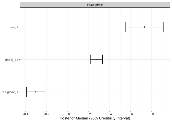
The section Fixed Effects provides information about the
fixed effects in the model, i.e., \(\gamma_{0,
\mu_1}\), \(\gamma_{0,
\phi_{(1)11}}\), and \(\gamma_{0,\ln(\sigma^2_{\zeta_{1}})}\) in
the above formula. For example, the posterior mean of the autoregressive
effect parameter phi(1)_11 is estimated at .27 with
95%-credible interval [.22, .33]. The log variance of the innovations
\(\zeta_{1t}\) is estimated at
-.30.
The section Random Effects SDs shows standard deviations
of the random effects \(\upsilon_{\mu_{1},i}\), \(\upsilon_{\phi_{(1)11},i}\), and \(\upsilon_{\ln(\sigma^2_{\zeta_{1}}),i}\).
The section Random Effects Correlations shows correlations
between random effects. For example, while random effects of the person
mean \(\upsilon_{\mu_{1},i}\) and the
autoregressive effect \(\upsilon_{\phi_{(1)11},i}\) display nearly
no correlation, 0.01, there is a positive correlation between the person
mean and log innovation variance, 0.22. This indicates that individuals
with a higher person mean in the variable Y1 also tend to
have a higher innovation variance.
The parameter estimates can also be plotted with the
mtls_plot()-function. By default, forest plots of model
parameters are produced. The what-argument controls what
parameter types are plotted (e.g., fixed effects, random effect standard
deviations, and other).
mlts_plot(ar1_fit, type = "fe", what = "Fixed effect")