MultiTraits is a comprehensive R package designed for advanced analysis and visualization of multidimensional plant traits. It provides a standardized workflow and intuitive visualization tools, streamlining the exploration of complex trait relationships for researchers, educators, and students. The package integrates four key analytical modules: Competitors–Stress Tolerators–Ruderals (CSR) strategy analysis, Leaf–Height–Seed (LHS) strategy analysis, Niche Periodic Table (NPT) analysis, and Plant Trait Network (PTN) analysis. These modules offer complementary perspectives, fostering a more comprehensive understanding of multidimensional trait variation patterns in plants. This tutorial aims to guide users through the core functionalities and practical applications of the MultiTraits package. Through hands-on demonstrations, we show how these analytical modules can be used to explore multidimensional relationships among plant traits, including essential steps in data preparation, analysis workflows, and results visualization.

{r,class.source = 'fold-show'} install.packages("MultiTraits")
{r,class.source = 'fold-show'} if (!requireNamespace("devtools", quietly = TRUE)) {install.packages("devtools")} devtools::install_github("biodiversity-monitoring/MultiTraits")
| Module | Function | Description |
|---|---|---|
| CSR Module | CSR() |
Classifies plant species’ CSR ecological strategies based on leaf traits (LA, LDMC, and SLA) using the Pierce et al. (2017) method. |
CSR_hodgson() |
Implements the Hodgson et al. (1999) method for CSR classification. | |
CSR_plot() |
Provides advanced ternary plot visualizations for CSR analysis to explore plant adaptation to different environments. | |
| LHS Module | LHS() |
Analyzes LHS strategies using SLA, plant height, and seed mass. |
LHS_plot() |
Visualizes three-dimensional trait distributions in LHS space. | |
LHS_strategy_scheme() |
Classifies strategies based on the LHS scheme. | |
| NPT Module | NPT_discrete() |
Supports discrete niche classification schemes. Performs PCA and clustering (CART or K-means) to group species within each dimension. |
NPT_discrete_plot() |
Visualizes the discrete niche classification scheme. | |
NPT_continuous() |
Supports continuous niche classification schemes. Performs a hierarchical PCA approach. | |
NPT_continuous_plot() |
Visualizes the results of the continuous niche classification. | |
| PTN Module | PTN_corr() |
Offers correlation computation and visualization for trait networks. |
PTN() |
Generates trait correlation networks. | |
PTN_metrics() |
Quantifies network metrics for trait networks. | |
PTN_plot() |
Visualizes the trait network graph. | |
| PTMN Module | PTMN() |
Constructs trait multilayer networks. |
PTMN_metrics() |
Calculates metrics for trait multilayer networks. | |
PTMN_plot() |
Visualizes trait multilayer networks. |
The package includes a built-in example dataset called PFF that can be loaded as follows:
{r,class.source = 'fold-show'} library(MultiTraits) data(PFF) # View the structure of the datasets head(PFF)
The PFF dataset contains trait measurements for plant species found in pine forests, with the following variables:
Height: Maximum plant height (cm)
Leaf_area: Leaf area (mm2)
LDMC: Leaf dry matter content (%)
SLA: Specific leaf area (mm2/mg)
SRL: Specific root length (m/g)
SeedMass: Seed mass (mg)
FltDate: Mean flowering date (Julian day)
FltDur: Mean flowering duration (days)
k_value: Decomposition decay constant, where proportion of original mass remaining = exp(- k-value*0.926)
Leaf_Cmass: Leaf carbon content (%)
Leaf_Nmass: Leaf nitrogen content (%)
Leaf_CN: Leaf carbon/nitrogen ratio
Leaf_Pmass: Leaf phosphorus content (%)
Leaf_NP: Leaf nitrogen/phosphorus ratio
Leaf_CP: Leaf carbon/phosphorus ratio
Root_Cmass: Root carbon content (%)
Root_Nmass: Root nitrogen content (%)
Root_CN: Root carbon/nitrogen ratio
The CSR (Competitor–Stress-Tolerator–Ruderal) strategy, initially conceptualized by Grime (1974), classifies plants based on their ecological strategies, which are influenced by environmental factors such as competition, stress, and disturbance. The MultiTraits package offers two approaches for CSR analysis: the method proposed by Hodgson et al. (1999) and the method developed by Pierce et al. (2017). The Pierce method, used here, employs leaf area (LA), leaf dry matter content (LDMC), and specific leaf area (SLA) to classify species. The CSR_plot() function visualizes the results in a ternary plot, showing species’ positions based on their relative C, S, and R strategy proportions. This aids in understanding plant functional classification and predicting responses to environmental changes.
```{r,class.source = ‘fold-show’} # Load packages library(MultiTraits) # Load the PFF dataset data(PFF) head(PFF)
csr_traits <- data.frame(LA=PFF\(Leaf_area, LDMC=PFF\)LDMC, SLA=PFF\(SLA) rownames(csr_traits) <- PFF\)species head(csr_traits)
csr_result <- CSR(csr_traits) head(csr_result)
CSR_plot(csr_result)
### LHS Strategy
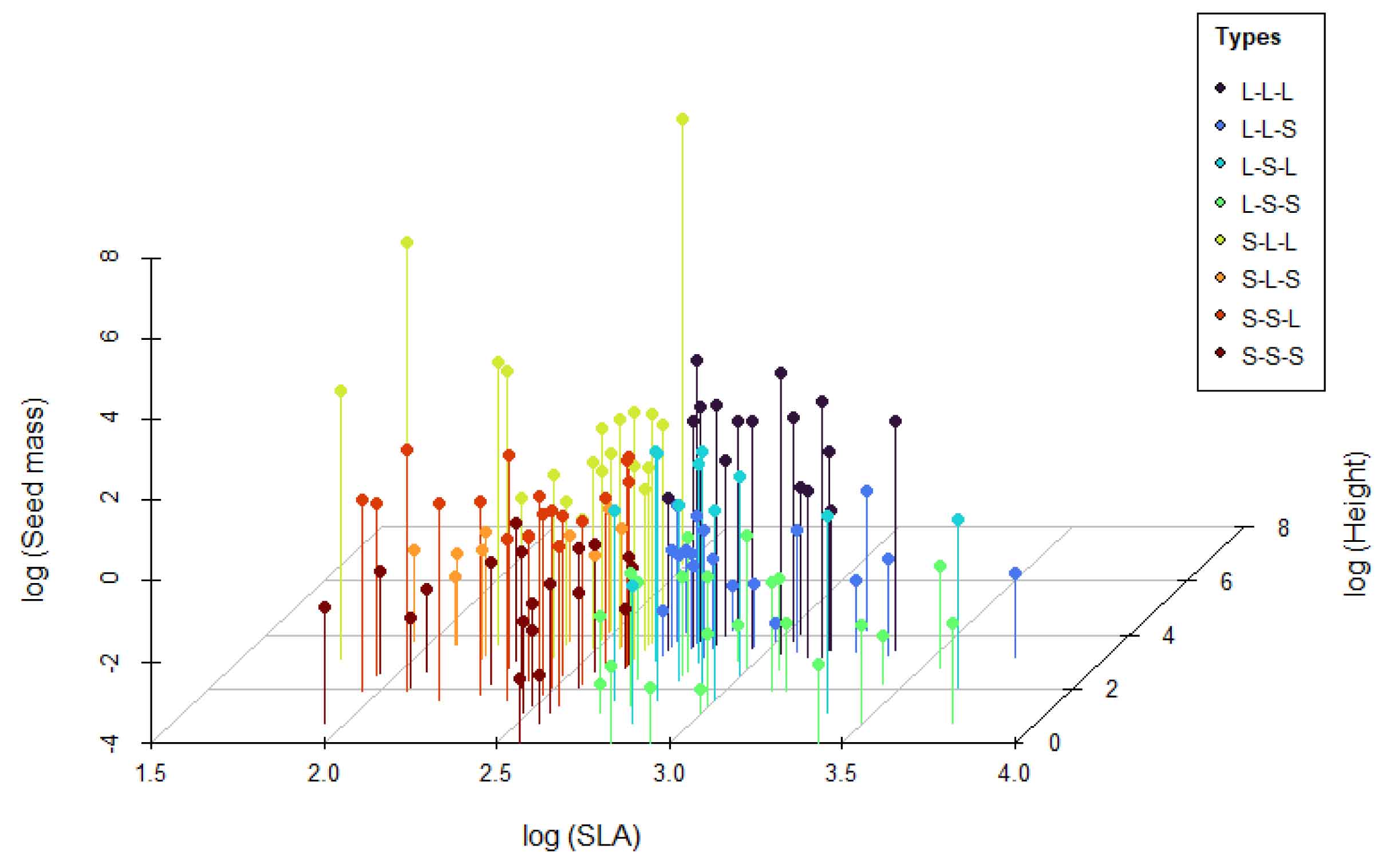
The Leaf--Height--Seed (LHS) scheme, proposed by Westoby (1998), classifies plant species based on specific leaf area (SLA), canopy height at maturity, and seed mass. These three traits reflect trade-offs in resource acquisition, spatial occupation, and reproductive investment. The MultiTraits package implements the LHS scheme by positioning species in a three-dimensional trait space using log-transformed trait values. This continuous space is then divided into eight discrete strategy types (e.g., S--S--S, L--L--L) based on median trait values, representing different trade-offs in growth, competition, and survival. The LHS_plot() function visualizes these strategies in 3D space, while LHS_strategy_scheme() provides a reference key for interpreting the strategy types.
```{r,class.source = 'fold-show'}
# Load packages
library(MultiTraits)
# Load the PFF dataset
data(PFF)
head(PFF)
# Create a data frame with the LHS traits
lhs_traits <- PFF[, c("SLA", "Height", "SeedMass")]
rownames(lhs_traits) <- PFF$species
head(lhs_traits)
# Perform LHS analysis
lhs_result <- LHS(lhs_traits)
head(lhs_result)
table(lhs_result$LHS_strategy)
# Create a visualization plot of the LHS analysis results
LHS_plot(lhs_result, group = "LHS_strategy", show_cube = TRUE)
# Display the LHS strategy scheme diagram
LHS_strategy_scheme()
The Niche Periodic Table (NPT) framework systematically describes and predicts species functions by identifying recurring trait combinations driven by convergent evolution. Within the MultiTraits R package, the NPT module offers both discrete and continuous classification schemes. The NPT_discrete() function categorizes species into distinct niche groups using PCA and clustering, with NPT_discrete_plot() visualizing the results. For continuous classification, NPT_continuous() performs hierarchical PCA to create a two-dimensional ordination space, while NPT_continuous_plot() visualizes these integrated niche patterns.
```{r,class.source = ‘fold-show’} # Load packages library(MultiTraits) # Load and prepare data data(PFF) rownames(PFF) <- PFF$species PFF_traits <- PFF[, c(“SLA”, “SRL”, “Leaf_Nmass”, “Root_Nmass”,“Height”, “Leaf_CN”, “Root_CN”,“SeedMass”, “FltDate”, “FltDur”)] # Perform log transformation of data and remove missing values PFF_traits <- log(na.omit(PFF_traits)) head(PFF_traits)
dimension <- list( Grow = c(“SLA”, “SRL”, “Leaf_Nmass”, “Root_Nmass”), Survive = c(“Height”, “Leaf_CN”, “Root_CN”), Reproductive = c(“SeedMass”, “FltDate”, “FltDur”) )
set.seed(123) discrete_result <- NPT_discrete(data = PFF_traits, dimension = dimension) discrete_result NPT_discrete_plot(discrete_result$niche_classification)
continuous_result <- NPT_continuous(data = PFF_traits, dimension = dimension) continuous_result NPT_continuous_plot(continuous_result$result)

### Plant Trait Network
Plant Trait Networks (PTNs) provide a framework for understanding complex interdependencies among plant traits by treating traits as nodes and their associations as edges within a network. The PTN module, implemented as described by He et al. (2020), offers functions to calculate correlations (PTN_corr()), generate networks (PTN()), quantify network metrics (PTN_metrics()), and visualize networks (PTN_plot()). The package supports phylogenetic correction to account for species' shared evolutionary history. Significant correlations are selected based on defined thresholds, and network metrics, including both node-level and network-level parameters, are used to analyze trait interdependence.
```{r,class.source = 'fold-show'}
# Load packages
library(MultiTraits)
# Load and prepare data
data(PFF)
rownames(PFF) <- PFF$species
PFF_traits <- PFF[, c("Leaf_area","LDMC","SLA", "Leaf_Cmass","Leaf_Nmass",
"Leaf_CN","Leaf_Pmass", "Leaf_NP","Leaf_CP")]
# Perform log transformation of data and remove missing values
PFF_traits <- log(na.omit(PFF_traits))
head(PFF_traits)
data(PFF_tree)
PFF_tree
# Calculate trait correlations using specified thresholds
PTN_corr(traits_matrix=PFF_traits, rThres = 0.2, pThres = 0.05,method = "pearson",
phylo_correction = TRUE,phylo_tree = PFF_tree)
# Perform Trait Network (TN) analysis
PTN_phylo_result <- PTN(traits_matrix = PFF_traits,
rThres = 0.2,
pThres = 0.05,
method = "pearson",
phylo_correction = TRUE,
phylo_tree = PFF_tree)
# Calculate network metrics for the trait network
PTN_metrics(PTN_phylo_result)
set.seed(22)
# Create visualization plots of the trait network
PTN_plot(PTN_phylo_result, style = 1, vertex.size = 20, vertex.label.cex = 0.6)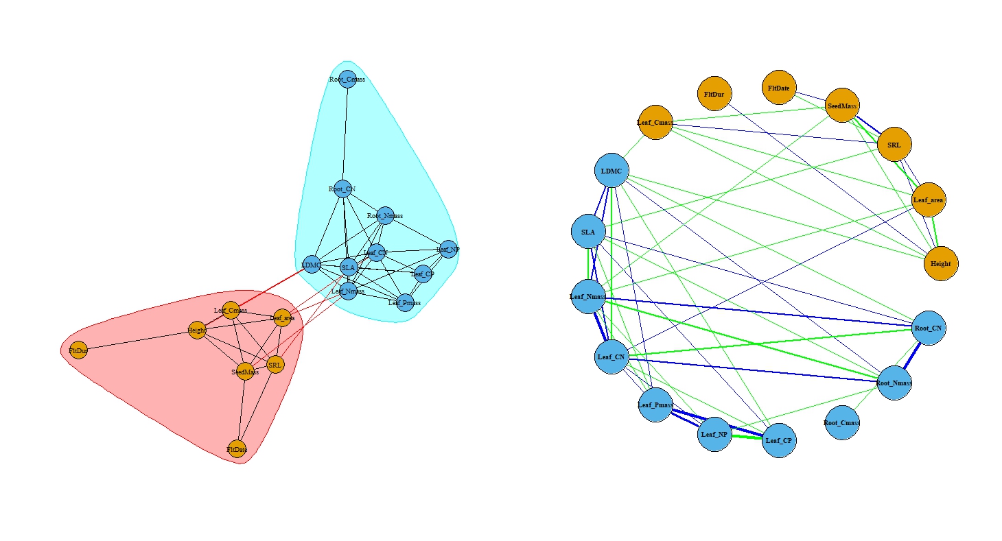
Plant Trait Multilayer Networks (PTMNs) provide an innovative framework for understanding multidimensional plant trait coordination, addressing the limitations of traditional, single-layer plant trait networks (PTNs). As outlined by He et al. (2026), this approach systematically organizes traits into distinct layers based on organs or functional systems (e.g., leaves, stems, roots). A key strength of PTMNs is the ability to differentiate between intralayer edges, which represent relationships within a single system, and interlayer edges, which capture the crucial coordination between different systems. The MultiTraits PTMN module implements this framework with functions to construct networks (PTMN()), calculate specialized multilayer metrics such as interlayer degree and module association (PTMN_metrics()), and create visualizations that clearly distinguish layer structure (PTMN_plot()). This methodology is powerful for identifying key traits that integrate whole-plant functioning and for revealing complex strategies of plant adaptation.
```{r,class.source = ‘fold-show’} # Load packages library(MultiTraits) # Load and prepare data data(forest_invader_traits) traits <- forest_invader_traits[, 6:73]
layers <- list( shoot_dynamics = c(“LeafDuration”, “LeafFall50”, “LeafRate_max”, “Chl_shade50”, “LAgain”, “FallDuration”, “LeafOut”, “Chl_sun50”, “EmergeDuration”, “LeafTurnover”), leaf_structure = c(“PA_leaf”, “Mass_leaf”, “Lifespan_leaf”, “Thick_leaf”, “SLA”, “Lobe”, “LDMC”, “Stomate_size”, “Stomate_index”), leaf_metabolism = c(“J_max”, “Vc_max”, “Asat_area”, “CC_mass”, “LSP”, “AQY”, “CC_area”, “Rd_area”, “Asat_mass”, “WUE”, “Rd_mass”, “PNUE”), leaf_chemistry = c(“N_area”, “Chl_area”, “DNA”, “Phenolics”, “Cellulose”, “N_mass”, “N_litter”, “Chl_ab”, “Chl_mass”, “N_res”, “C_litter”, “C_area”, “C_mass”, “Ash”, “Lignin”, “Solubles”, “Decomp_leaf”, “Hemi”), root = c(“NPP_root”, “SS_root”, “SRL”, “RTD”, “RDMC”, “NSC_root”, “Decomp_root”, “Starch_root”, “C_root”, “N_root”, “Lignin_root”), stem = c(“Latewood_diam”, “Metaxylem_diam”, “Earlywood_diam”, “NSC_stem”, “Vessel_freq”, “SS_stem”, “Cond_stem”, “Starch_stem”) )
ptmn_edges <- PTMN(traits, layers_list = layers, method = “pearson”)
PTMN_metrics(ptmn_edges)
set.seed(42) # Create a visualization of the PTMN PTMN_plot(ptmn_edges, style = 1, vertex.size = 8, vertex.label.cex = 0.5, edge.width = 2, show.legend = FALSE) ```

If you use MultiTraits in your research, please cite the
following paper(s). This is the best way to support the development and
maintenance of the package.
For the overall MultiTraits framework and its
core modules (CSR, LHS, NPT, PTN), please cite our Ecography
paper:
He, Y., Liu, Z., Lai, J. & Mao, L. (2026). ‘MultiTraits’: an integrated R package for analysis and visualization of multidimensional plant traits. Ecography, e08026. https://doi.org/10.1002/ecog.08026
If you specifically use the Plant Trait Multilayer Network (PTMN) module, please cite our New Phytologist paper as well:
He, Y., Xia, Y., Liu, Z., Yang, R., Lai, J. & Mao, L. (2026). Plant trait multilayer networks: a new framework for understanding multidimensional plant trait coordination. New Phytologist, 249: 2115-2124. https://doi.org/10.1111/nph.70785