![]()
![]()
The fluxible R package is made to transform any dataset
of gas concentration over time measured with closed loop chamber systems
into a gas flux dataset.
Thanks to its flexibility, it works for all kinds of field setup (manual
or automated chambers, tents, soil respiration chambers, …) and data
collection strategies (separated files for each measurement vs
continuous logging, variable vs constant chamber volume, variable vs
constant measurement length, …). It is organized as a toolbox with one
function per steps, which offers a lot of freedom and backwards
compatibility for ongoing projects. If environmental data were recorded
simultaneously (photosynthetically active radiation, soil temperature,
…), they can also be processed (mean, sum or median), with the same
focus window as the flux estimate.
The goal of fluxible is to provide a workflow that
removes individual evaluation of each flux, reduces risk of bias, and
makes it reproducible. Users set specific data quality standards and
selection parameters as function arguments that are applied to the
entire dataset. fluxible offers different methods to
estimate fluxes: linear, quadratic, exponential (Zhao et al.,
2018), and the original HM model (Hutchinson and Mosier, 1981; Pedersen
et al., 2010). The kappamax method (Hüppi et al.,
2018) is also included, at the quality control step. The package runs
the calculations automatically, without prompting the user to take
decisions mid-way, and provides quality flags and plots at the end of
the process for a visual check.
This makes it easy to use with large flux datasets and to integrate
into a reproducible and automated data processing pipeline such as the
targets R
package (Landau, 2021). Using the fluxible R package
makes the workflow reproducible, increases compatibility across studies,
and is more time efficient.
For a visual overview of the package, see the poster.
fluxible can be installed from CRAN.
install.packages("fluxible")You can install the development version of fluxible from
the GitHub
repo with:
# install.packages("devtools")
devtools::install_github("plant-functional-trait-course/fluxible")library(fluxible)
conc_df <- flux_match(
co2_df_short,
record_short,
datetime,
start,
measurement_length = 220
)
slopes_df <- flux_fitting(
conc_df,
conc,
datetime,
fit_type = "exp_zhao18",
end_cut = 60
)
#> Cutting measurements...
#> Estimating starting parameters for optimization...
#> Optimizing fitting parameters...
#> Calculating fits and slopes...
#> Done.
slopes_flag_df <- flux_quality(
slopes_df,
conc
)
#>
#> Total number of measurements: 6
#>
#> ok 6 100 %
#> discard 0 0 %
#> zero 0 0 %
#> force_discard 0 0 %
#> start_error 0 0 %
#> no_data 0 0 %
#> force_ok 0 0 %
#> force_zero 0 0 %
#> force_lm 0 0 %
#> no_slope 0 0 %
flux_plot(
slopes_flag_df,
conc,
datetime,
f_ylim_lower = 390,
f_ylim_upper = 650,
facet_wrap_args = list(
ncol = 3,
nrow = 2,
scales = "free"
)
)
#> Plotting in progress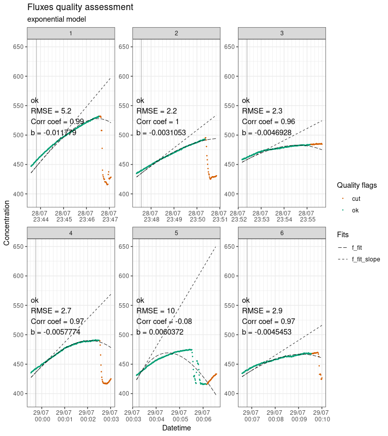
Output of flux_plot, showing fluxes plotted individually with diagnostics and quality flags.
fluxes_df <- flux_calc(
  slopes_flag_df,
  f_slope_corr,
  datetime,
  temp_air,
  conc_unit = "ppm",
  flux_unit = "mmol/m2/h",
  cols_keep = c("turfID", "type"),
  cols_ave = c("temp_soil", "PAR"),
  setup_volume = 24.575,
  atm_pressure = 1,
  plot_area = 0.0625
)
#> Cutting data according to 'keep_arg'...
#> Averaging air temperature for each flux...
#> Creating a df with the columns from 'cols_keep' argument...
#> Creating a df with the columns from 'cols_ave' argument...
#> Calculating fluxes...
#> R constant set to 0.082057 L * atm * K^-1 * mol^-1
#> Concentration was measured in ppm
#> Fluxes are in mmol/m2/h

fluxes_gpp <- flux_gpp(
  fluxes_df,
  type,
  datetime,
  id_cols = "turfID",
  cols_keep = c("temp_soil_ave")
)
#> Warning in flux_gpp(fluxes_df, type, datetime, id_cols = "turfID", cols_keep = c("temp_soil_ave")):
#>  NEE missing for measurement turfID: 156 AN2C 156

fluxes_gpp
#> # A tibble: 9 × 5
#>   datetime            type  f_flux temp_soil_ave turfID
#>   <dttm>              <chr>  <dbl>         <dbl> <chr>
#> 1 2022-07-28 23:43:25 ER     51.9           10.9 156 AN2C 156
#> 2 2022-07-28 23:47:12 GPP     9.72          10.7 74 WN2C 155
#> 3 2022-07-28 23:47:12 NEE    32.0           10.7 74 WN2C 155
#> 4 2022-07-28 23:52:00 ER     22.3           10.7 74 WN2C 155
#> 5 2022-07-28 23:59:22 GPP    -6.63          10.8 109 AN3C 109
#> 6 2022-07-28 23:59:22 NEE    44.3           10.8 109 AN3C 109
#> 7 2022-07-29 00:03:00 ER     50.9           10.5 109 AN3C 109
#> 8 2022-07-29 00:06:25 GPP    NA             12.2 29 WN3C 106
#> 9 2022-07-29 00:06:25 NEE 32.7 12.2 29 WN3C 106licoread R packageThe licoread
R package, developed in collaboration with LI-COR, provides an easy way to import
raw files from LI-COR gas analyzers as R objects that can be used
directly with the fluxible R package.
We are working on a tool to automatically select the window of the measurement on which to fit a model. This selection will be based on environmental variable, such as photosynthetically active radiation (PAR), or residuals.
So far fluxible works in fractional concentration (e. g.
ppm) and transforms it in mol when calculating the fluxes, using the
average temperature of the measurement. This has the advantage to work
even if the setup does not provide temperature for each gas
concentration data point. Recent setups provide temperature at the same
frequency as gas concentration, and this allows to transform the
concentration in mol/volume earlier in the process, accounting better
for temperature changes during the measurement. This will be implemented
in a future version of fluxible.
Joseph Gaudard, University of Bergen, Norway
Gaudard J, Telford RJ, Chacon-Labella J, Dawson HR, Enquist BJ,
Töpper JP, Trepel J, Vandvik V, Baumane M, Birkeli K, Holle MJM, Hupp
JR, Santos-Andrade PE, Satriawan TW, Halbritter AH.
“fluxible: An R package to process ecosystem gas fluxes
from closed-loop chambers in an automated and reproducible way” (2025).
Methods in Ecology and Evolution, doi:10.1111/2041-210X.70161.
Gaudard J, Telford RJ, Chacon-Labella J, Dawson HR, Enquist
BJ, Töpper JP, Trepel J, Vandvik V, Baumane M, Birkeli K, Holle
MJM, Hupp JR, Santos-Andrade PE, Satriawan TW, Halbritter AH.
“fluxible: An R package to process ecosystem gas fluxes
from closed-loop chambers in an automated and reproducible way”, Poster,
2025 AmeriFlux Annual Meeting, Tucson AZ, USA.
Gaudard J, Telford RJ, Chacon-Labella J, Dawson HR, Enquist BJ,
Töpper JP, Trepel J, Vandvik V, Baumane M, Birkeli K,
Holle MJM, Hupp JR, Santos-Andrade PE, Satriawan TW, Halbritter AH.
“fluxible: An R package to process ecosystem gas fluxes
from closed-loop chambers in an automated and reproducible way”, Poster,
ITEX Meeting 2025, Göteborg, Sweden.
Gaudard J, Trepel J, Dawson HR, Enquist B,
Halbritter AH, Mustri M, Niittynen P, Santos-Andrade PE, Töpper JP,
Vandvik V, and Telford RJ. “fluxible: an R package to
calculate ecosystem gas fluxes from closed loop chamber systems in a
reproducible and automated workflow”, Oral presentation, EGU General
Assembly 2025, Vienna, Austria, 27 Apr-2 May 2025, EGU25-12409, doi:10.5194/egusphere-egu25-12409.
Gaudard J, Dawson HR, Enquist B, Halbritter AH,
Mustri M, Niittynen P, Santos-Andrade PE, Töpper JP, Trepel J, Vandvik
V, and Telford RJ. “fluxible: an R package to calculate
ecosystem gas fluxes from closed loop chamber systems in a reproducible
and automated workflow”, Poster, LI-COR Connect 2025, Tucson AZ, USA,
24-27 Feb 2025.
Gaudard J, Telford R, Vandvik V, and Halbritter AH:
“fluxible: an R package to calculate ecosystem gas fluxes
in a reproducible and automated workflow”, Poster, EGU General Assembly
2024, Vienna, Austria, 14-19 Apr 2024, EGU24-956, doi:10.5194/egusphere-egu24-956.
fluxible builds on the earlier effort from the Plant
Functional Traits Course Community co2fluxtent
(Brummer et al., 2023).