
![]()

Efficient procedures for constrained likelihood estimation with truncated lasso penalty (Shen et al., 2010; Zhang 2010) for linear and generalized linear models.
Note: this is a repo for the version published on CRAN. Please check chunlinli/glmtlp for new features such as constrained likelihood inference, regression on summary data, memory efficiency, Gaussian graphical models, and more.
You can install the released version of glmtlp from CRAN with:
install.packages("glmtlp")The following are three examples which show you how to use
glmtlp to fit gaussian regression models:
library(glmtlp)
data("gau_data")
colnames(gau_data$X)[gau_data$beta != 0]
#> [1] "V1"  "V6"  "V10" "V15" "V20"
# Cross-Validation using TLP penalty
cv.fit <- cv.glmtlp(gau_data$X, gau_data$y, family = "gaussian", penalty = "tlp", ncores=2)
coef(cv.fit)[abs(coef(cv.fit)) > 0]
#> intercept V1 V6 V10 V15 V20
#> -0.009678041 1.240223517 0.883202180 0.725708239 1.125994003 0.981402236
plot(cv.fit)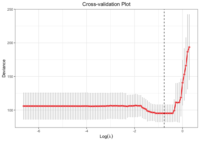
# Single Model Fit using TLP penalty
fit <- glmtlp(gau_data$X, gau_data$y, family = "gaussian", penalty = "tlp")
coef(fit, lambda = cv.fit$lambda.min)
#>    intercept           V1           V2           V3           V4           V5
#> -0.009678041  1.240223517  0.000000000  0.000000000  0.000000000  0.000000000
#>           V6           V7           V8           V9          V10          V11
#>  0.883202180  0.000000000  0.000000000  0.000000000  0.725708239  0.000000000
#>          V12          V13          V14          V15          V16          V17
#>  0.000000000  0.000000000  0.000000000  1.125994003  0.000000000  0.000000000
#>          V18          V19          V20
#>  0.000000000  0.000000000  0.981402236
predict(fit, X = gau_data$X[1:5, ], lambda = cv.fit$lambda.min)
#> [1]  0.1906465  2.2279723 -1.4256042  0.9313886 -2.8152522
plot(fit, xvar = "log_lambda", label = TRUE)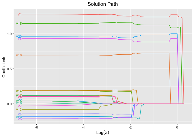
# Cross-Validation using L0 penalty
cv.fit <- cv.glmtlp(gau_data$X, gau_data$y, family = "gaussian", penalty = "l0", ncores=2)
coef(cv.fit)[abs(coef(cv.fit)) > 0]
#>    intercept           V1           V6          V10          V15          V20
#> -0.009687042  1.240319880  0.883378583  0.725607300  1.125958218  0.981544178
plot(cv.fit)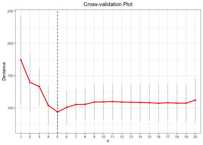
# Single Model Fit using L0 penalty
fit <- glmtlp(gau_data$X, gau_data$y, family = "gaussian", penalty = "l0")
coef(fit, kappa = cv.fit$kappa.min)
#>    intercept           V1           V2           V3           V4           V5
#> -0.009687042  1.240319880  0.000000000  0.000000000  0.000000000  0.000000000
#>           V6           V7           V8           V9          V10          V11
#>  0.883378583  0.000000000  0.000000000  0.000000000  0.725607300  0.000000000
#>          V12          V13          V14          V15          V16          V17
#>  0.000000000  0.000000000  0.000000000  1.125958218  0.000000000  0.000000000
#>          V18          V19          V20
#>  0.000000000  0.000000000  0.981544178
predict(fit, X = gau_data$X[1:5, ], kappa = cv.fit$kappa.min)
#> [1]  0.190596  2.228306 -1.425994  0.931749 -2.815322
plot(fit, xvar = "kappa", label = TRUE)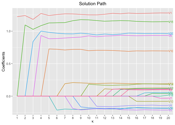
# Cross-Validation using L1 penalty
cv.fit <- cv.glmtlp(gau_data$X, gau_data$y, family = "gaussian", penalty = "l1", ncores=2)
coef(cv.fit)[abs(coef(cv.fit)) > 0]
#>   intercept          V1          V3          V4          V5          V6
#> -0.01185622  1.16222899 -0.06606911 -0.08387185 -0.06870578  0.79106593
#>          V8          V9         V10         V11         V14         V15
#>  0.01136376  0.01038075  0.62580166  0.10858744  0.08533479  1.04737369
#>         V19         V20
#> -0.11859786  0.86736897
plot(cv.fit)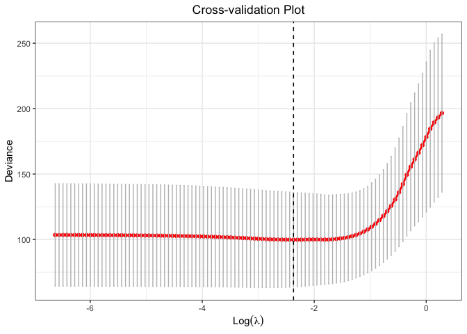
# Single Model Fit using L1 penalty
fit <- glmtlp(gau_data$X, gau_data$y, family = "gaussian", penalty = "l1")
coef(fit, lambda = cv.fit$lambda.min)
#>   intercept          V1          V2          V3          V4          V5
#> -0.01185622  1.16222899  0.00000000 -0.06606911 -0.08387185 -0.06870578
#>          V6          V7          V8          V9         V10         V11
#>  0.79106593  0.00000000  0.01136376  0.01038075  0.62580166  0.10858744
#>         V12         V13         V14         V15         V16         V17
#>  0.00000000  0.00000000  0.08533479  1.04737369  0.00000000  0.00000000
#>         V18         V19         V20
#>  0.00000000 -0.11859786  0.86736897
predict(fit, X = gau_data$X[1:5, ], lambda = cv.fit$lambda.min)
#> [1]  0.07112074  2.17093497 -1.09936871  0.46108771 -2.25111685
plot(fit, xvar = "lambda", label = TRUE)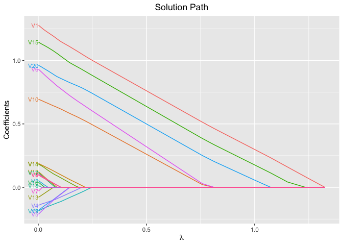
The following are three examples which show you how to use
glmtlp to fit logistic regression models:
data("bin_data")
colnames(bin_data$X)[bin_data$beta != 0]
#> [1] "V1"  "V6"  "V10" "V15" "V20"
# Cross-Validation using TLP penalty
cv.fit <- cv.glmtlp(bin_data$X, bin_data$y, family = "binomial", penalty = "tlp", ncores=2)
coef(cv.fit)[abs(coef(cv.fit)) > 0]
#> intercept V6 V20
#> -0.1347141 0.8256183 0.9940325
plot(cv.fit)
#> Warning: Removed 98 rows containing missing values or values outside the scale range
#> (`geom_line()`).
#> Warning: Removed 98 rows containing missing values or values outside the scale range
#> (`geom_point()`).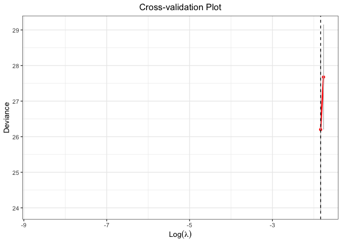
# Single Model Fit using TLP penalty
fit <- glmtlp(bin_data$X, bin_data$y, family = "binomial", penalty = "tlp")
coef(fit, lambda = cv.fit$lambda.min)
#>  intercept         V1         V2         V3         V4         V5         V6
#> -0.1347141  0.0000000  0.0000000  0.0000000  0.0000000  0.0000000  0.8256183
#>         V7         V8         V9        V10        V11        V12        V13
#>  0.0000000  0.0000000  0.0000000  0.0000000  0.0000000  0.0000000  0.0000000
#>        V14        V15        V16        V17        V18        V19        V20
#>  0.0000000  0.0000000  0.0000000  0.0000000  0.0000000  0.0000000  0.9940325
predict(fit, X = bin_data$X[1:5, ], type = "response", lambda = cv.fit$lambda.min)
#> [1] 0.42562483 0.89838483 0.09767039 0.90898462 0.20822294
plot(fit, xvar = "log_lambda", label = TRUE)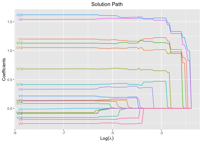
# Cross-Validation using L0 penalty
cv.fit <- cv.glmtlp(bin_data$X, bin_data$y, family = "binomial", penalty = "l0", ncores=2)
coef(cv.fit)[abs(coef(cv.fit)) > 0]
#>  intercept         V6        V20
#> -0.1347137  0.8256471  0.9940180
plot(cv.fit)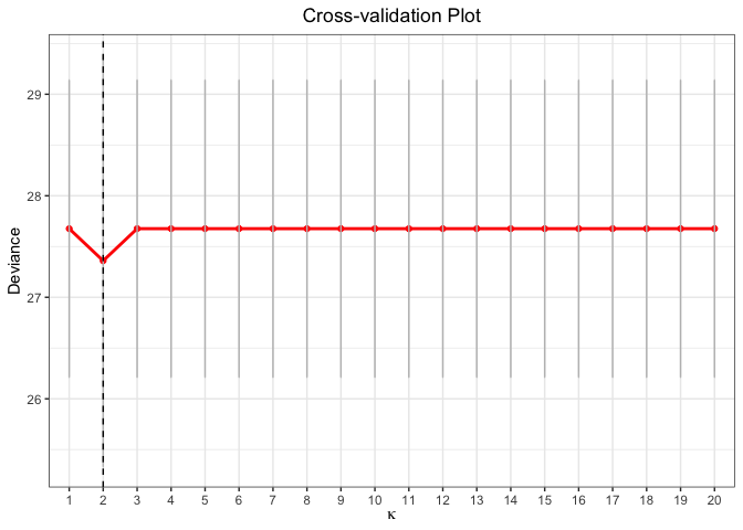
# Single Model Fit using L0 penalty
fit <- glmtlp(bin_data$X, bin_data$y, family = "binomial", penalty = "l0")
coef(fit, kappa = cv.fit$kappa.min)
#>  intercept         V1         V2         V3         V4         V5         V6
#> -0.1347137  0.0000000  0.0000000  0.0000000  0.0000000  0.0000000  0.8256471
#>         V7         V8         V9        V10        V11        V12        V13
#>  0.0000000  0.0000000  0.0000000  0.0000000  0.0000000  0.0000000  0.0000000
#>        V14        V15        V16        V17        V18        V19        V20
#>  0.0000000  0.0000000  0.0000000  0.0000000  0.0000000  0.0000000  0.9940180
predict(fit, X = bin_data$X[1:5, ], kappa = cv.fit$kappa.min)
#> [1] -0.2996886  2.1793764 -2.2234461  2.3012922 -1.3357999
plot(fit, xvar = "kappa", label = TRUE)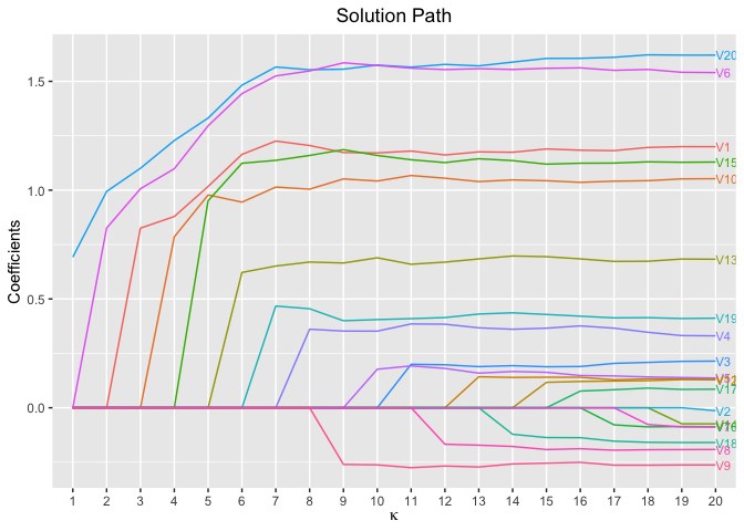
# Cross-Validation using L1 penalty
cv.fit <- cv.glmtlp(bin_data$X, bin_data$y, family = "binomial", penalty = "l1", ncores=2)
coef(cv.fit)[abs(coef(cv.fit)) > 0]
#>   intercept          V1          V3          V4          V5          V6
#> -0.04597434  0.74281436  0.04345031  0.15993696  0.05100859  0.98672196
#>          V8          V9         V10         V13         V15         V19
#> -0.04488821 -0.06456282  0.66422939  0.33826482  0.69062166  0.23686317
#>         V20
#>  1.01116571
plot(cv.fit)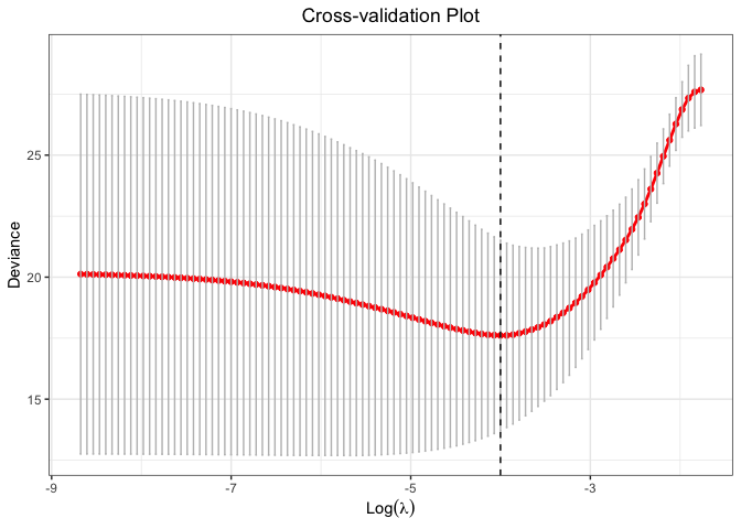
# Single Model Fit using L1 penalty
fit <- glmtlp(bin_data$X, bin_data$y, family = "binomial", penalty = "l1")
coef(fit, lambda = cv.fit$lambda.min)
#>   intercept          V1          V2          V3          V4          V5
#> -0.04597434  0.74281436  0.00000000  0.04345031  0.15993696  0.05100859
#>          V6          V7          V8          V9         V10         V11
#>  0.98672196  0.00000000 -0.04488821 -0.06456282  0.66422939  0.00000000
#>         V12         V13         V14         V15         V16         V17
#>  0.00000000  0.33826482  0.00000000  0.69062166  0.00000000  0.00000000
#>         V18         V19         V20
#>  0.00000000  0.23686317  1.01116571
predict(fit, X = bin_data$X[1:5, ], type = "response", lambda = cv.fit$lambda.min)
#> [1] 0.35132374 0.90851038 0.03822033 0.93657911 0.03253188
plot(fit, xvar = "lambda", label = TRUE)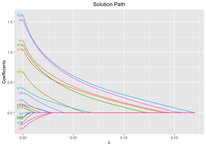
If you find this project useful, please consider citing
@article{
    author = {Chunlin Li, Yu Yang, Chong Wu, Xiaotong Shen, Wei Pan},
    title = {{glmtlp: An R package for truncated Lasso penalty}},
    year = {2022}
}Li, C., Shen, X., & Pan, W. (2021). Inference for a large directed graphical model with interventions. arXiv preprint arXiv:2110.03805. https://arxiv.org/abs/2110.03805.
Shen, X., Pan, W., & Zhu, Y. (2012). Likelihood-based selection and sharp parameter estimation. Journal of the American Statistical Association, 107(497), 223-232. https://doi.org/10.1080/01621459.2011.645783.
Shen, X., Pan, W., Zhu, Y., & Zhou, H. (2013). On constrained and regularized high-dimensional regression. Annals of the Institute of Statistical Mathematics, 65(5), 807-832. https://doi.org/10.1007/s10463-012-0396-3.
Tibshirani, R., Bien, J., Friedman, J., Hastie, T., Simon, N., Taylor, J., & Tibshirani, R. J. (2012). Strong rules for discarding predictors in lasso‐type problems. Journal of the Royal Statistical Society: Series B (Statistical Methodology), 74(2), 245-266. https://doi.org/10.1111/j.1467-9868.2011.01004.x.
Yang, Y. & Zou, H. A coordinate majorization descent algorithm for l1 penalized learning. Journal of Statistical Computation and Simulation 84.1 (2014): 84-95. https://doi.org/10.1080/00949655.2012.695374.
Zhu, Y., Shen, X., & Pan, W. (2020). On high-dimensional constrained maximum likelihood inference. Journal of the American Statistical Association, 115(529), 217-230. https://doi.org/10.1080/01621459.2018.1540986.
Zhu, Y. (2017). An augmented ADMM algorithm with application to the generalized lasso problem. Journal of Computational and Graphical Statistics, 26(1), 195-204. https://doi.org/10.1080/10618600.2015.1114491.
Part of the code is adapted from glmnet, ncvreg, and biglasso.
Warm thanks to the authors of above open-sourced softwares.