![]()
![]()
ggchangepoint provides a unified tidy interface to changepoint
analysis in R. It wraps multiple detection engines (changepoint,
changepoint.np, ecp, wbs, breakfast, not, mosum, fpop, IDetect) behind a
consistent S3 result class (ggcpt) with
broom-style methods (tidy(),
glance(), augment()), ggplot2
integration via autoplot() and custom geoms, and a full
method-comparison, evaluation, simulation, and visualisation
toolkit.
The engines beyond changepoint,
changepoint.np, and ecp are optional
(Suggests); install the ones you need. The original 0.1.0
functions (cpt_wrapper(), ecp_wrapper(),
ggcptplot(), ggecpplot()) continue to work
unchanged.
Install the released version from CRAN:
install.packages("ggchangepoint")Or the development version from GitHub:
# install.packages("devtools")
devtools::install_github("PursuitOfDataScience/ggchangepoint")library(ggchangepoint)
library(ggplot2)Generate a series with a mean shift:
set.seed(2022)
x <- c(rnorm(100, 0, 1), rnorm(100, 10, 1))
Detect changepoints with the unified cpt_detect():
res <- cpt_detect(x, method = "pelt", change_in = "mean")
res
#> ggcpt (changepoint detection result)
#>   Method:          pelt
#>   Change in:       mean
#>   Changepoints found: 1
#>   CP convention:   left
#>   Penalty:         MBIC = NA
#>   Series length:   200
#>
#> Changepoints:
#> # A tibble: 1 × 2
#>      cp cp_value
#>   <int>    <dbl>
#> 1   100    0.467
The result is a ggcpt S3 object. Print it to see the
changepoints, or use tidy(), glance(), and
augment():
tidy(res)
#> # A tibble: 1 × 2
#>      cp cp_value
#>   <int>    <dbl>
#> 1   100    0.467
glance(res)
#> # A tibble: 1 × 9
#>       n n_changepoints method change_in penalty_type penalty_value cp_convention
#>   <int>          <int> <chr>  <chr>     <chr>                <dbl> <chr>
#> 1   200              1 pelt   mean      MBIC                    NA left
#> # ℹ 2 more variables: total_cost <dbl>, runtime <dbl>
Visualise with autoplot():
autoplot(res)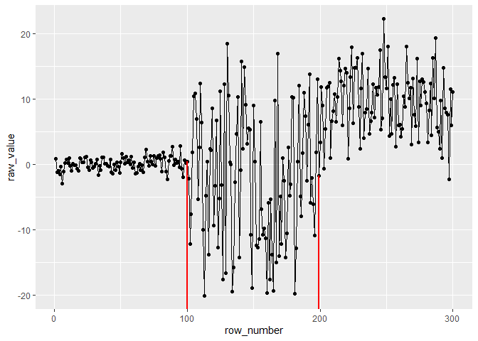
cpt_detect() dispatches to any supported method by
name:
cpt_detect(x, method = "binseg", change_in = "mean")
#> ggcpt (changepoint detection result)
#>   Method:          binseg
#>   Change in:       mean
#>   Changepoints found: 1
#>   CP convention:   left
#>   Penalty:         MBIC = NA
#>   Series length:   200
#>
#> Changepoints:
#> # A tibble: 1 × 2
#>      cp cp_value
#>   <dbl>    <dbl>
#> 1   100    0.467
cpt_detect(x, method = "wbs", change_in = "mean")
#> ggcpt (changepoint detection result)
#>   Method:          wbs
#>   Change in:       mean
#>   Changepoints found: 1
#>   CP convention:   left
#>   Penalty:         sSIC = NA
#>   Series length:   200
#>
#> Changepoints:
#> # A tibble: 1 × 2
#>      cp cp_value
#>   <int>    <dbl>
#> 1   100    0.467
cpt_detect(x, method = "fpop", change_in = "mean")
#> ggcpt (changepoint detection result)
#>   Method:          fpop
#>   Change in:       mean
#>   Changepoints found: 1
#>   CP convention:   left
#>   Penalty:         Manual = 10.5966347330961
#>   Series length:   200
#>
#> Changepoints:
#> # A tibble: 1 × 2
#>      cp cp_value
#>   <int>    <dbl>
#> 1   100    0.467
Use cpt_methods() to see all available and planned
methods with their engine packages and installation status:
cpt_methods()
#> # A tibble: 26 × 6
#>    method   change_in          engine         status    target_release installed
#>    <chr>    <chr>              <chr>          <chr>     <chr>          <lgl>
#>  1 pelt     mean, var, meanvar changepoint    available <NA>           TRUE
#>  2 binseg   mean, var, meanvar changepoint    available <NA>           TRUE
#>  3 segneigh mean, var, meanvar changepoint    available <NA>           TRUE
#>  4 amoc     mean, var, meanvar changepoint    available <NA>           TRUE
#>  5 np       distribution       changepoint.np available <NA>           TRUE
#>  6 ecp      distribution       ecp            available <NA>           TRUE
#>  7 fpop     mean               fpop           available <NA>           TRUE
#>  8 wbs      mean               wbs            available <NA>           TRUE
#>  9 wbs2     mean               breakfast      available <NA>           TRUE
#> 10 not      mean, var, slope   not            available <NA>           TRUE
#> # ℹ 16 more rowsggcpt_compare(x, methods = c("pelt", "binseg", "fpop", "wbs"))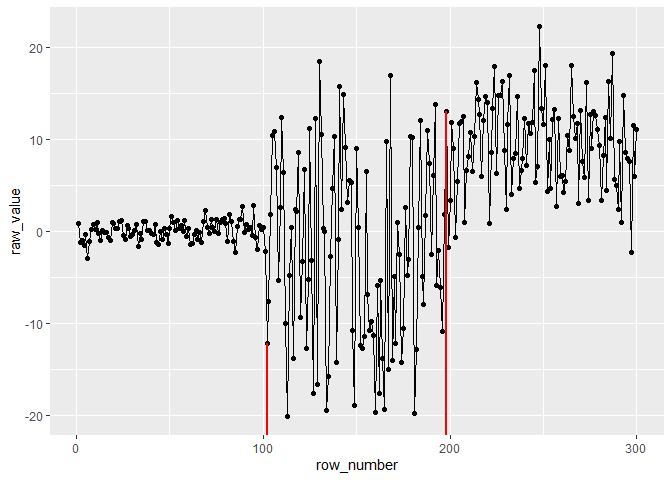
For a numeric summary, use ggcpt_compare_table():
ggcpt_compare_table(x, methods = c("pelt", "binseg", "fpop", "wbs"))
#> # A tibble: 4 × 3
#>   method    cp cp_value
#>   <chr>  <dbl>    <dbl>
#> 1 pelt     100    0.467
#> 2 binseg   100    0.467
#> 3 fpop     100    0.467
#> 4 wbs 100 0.467When ground truth changepoints are known, compute accuracy metrics:
cpt_metrics(pred = c(100), truth = c(100), n = 200)
#> # A tibble: 1 × 12
#>       n n_pred n_truth precision recall    f1 covering hausdorff rand_index
#>   <int>  <int>   <int>     <dbl>  <dbl> <dbl>    <dbl>     <dbl>      <dbl>
#> 1   200      1       1         1      1     1        1         0          1
#> # ℹ 3 more variables: annotation_error <int>, mae_matched <dbl>,
#> # rmse_matched <dbl>dat <- cpt_simulate(200, changepoints = c(100), change_in = "mean",
params = c(0, 10), sd = 1)
attributes(dat)$true_changepoints
#> [1] 100An alias rcpt() is provided for compatibility. Built-in
test signals include signal_blocks(),
signal_fms(), signal_mix(),
signal_teeth(), and signal_stairs().
Use cpt_penalty() to construct penalty values for use
with detection methods:
cpt_penalty("BIC", n = 200)
#> [1] 5.298317
cpt_penalty("AIC", n = 200)
#> [1] 2
cpt_penalty("Manual", value = 10)
#> [1] 10For fine-grained control, each detection engine has its own wrapper
that returns a ggcpt object directly:
fpop_wrapper(x, penalty = 2 * log(200))
#> ggcpt (changepoint detection result)
#>   Method:          fpop
#>   Change in:       mean
#>   Changepoints found: 1
#>   CP convention:   left
#>   Penalty:         Manual = 10.5966347330961
#>   Series length:   200
#>
#> Changepoints:
#> # A tibble: 1 × 2
#>      cp cp_value
#>   <int>    <dbl>
#> 1   100    0.467
wbs_wrapper(x, n_intervals = 2000)
#> ggcpt (changepoint detection result)
#>   Method:          wbs
#>   Change in:       mean
#>   Changepoints found: 1
#>   CP convention:   left
#>   Penalty:         sSIC = NA
#>   Series length:   200
#>
#> Changepoints:
#> # A tibble: 1 × 2
#>      cp cp_value
#>   <int>    <dbl>
#> 1   100    0.467
wbs2_wrapper(x)
#> ggcpt (changepoint detection result)
#>   Method:          wbs2
#>   Change in:       mean
#>   Changepoints found: 1
#>   CP convention:   left
#>   Penalty:         SDLL = NA
#>   Series length:   200
#>
#> Changepoints:
#> # A tibble: 1 × 2
#>      cp cp_value
#>   <int>    <dbl>
#> 1   100    0.467
not_wrapper(x, contrast = "pcwsConstMean")
#> ggcpt (changepoint detection result)
#>   Method:          not
#>   Change in:       mean
#>   Changepoints found: 1
#>   CP convention:   left
#>   Penalty:         sSIC = NA
#>   Series length:   200
#>
#> Changepoints:
#> # A tibble: 1 × 2
#>      cp cp_value
#>   <int>    <dbl>
#> 1   100    0.467
mosum_wrapper(x)
#> ggcpt (changepoint detection result)
#>   Method:          mosum
#>   Change in:       mean
#>   Changepoints found: 1
#>   CP convention:   left
#>   Penalty:         threshold = critical.value
#>   Series length:   200
#>
#> Changepoints:
#> # A tibble: 1 × 2
#>      cp cp_value
#>   <int>    <dbl>
#> 1   100    0.467
idetect_wrapper(x)
#> ggcpt (changepoint detection result)
#>   Method:          IDetect
#>   Change in:       mean
#>   Changepoints found: 1
#>   CP convention:   left
#>   Penalty:         threshold = NA
#>   Series length:   200
#>
#> Changepoints:
#> # A tibble: 1 × 2
#>      cp cp_value
#>   <int>    <dbl>
#> 1   100    0.467
tguh_wrapper(x)
#> ggcpt (changepoint detection result)
#>   Method:          tguh
#>   Change in:       mean
#>   Changepoints found: 1
#>   CP convention:   left
#>   Penalty:         threshold = NA
#>   Series length:   200
#>
#> Changepoints:
#> # A tibble: 1 × 2
#>      cp cp_value
#>   <int>    <dbl>
#> 1 100 0.467The package provides composable ggplot2 layers for changepoint visualisation:
library(ggplot2)

# Use geom_changepoint as a standalone layer
cp_tbl <- tidy(cpt_detect(x, method = "pelt", change_in = "mean"))
ggplot(data.frame(index = seq_along(x), value = x), aes(index, value)) +
  geom_line() +
  geom_changepoint(data = cp_tbl, aes(xintercept = cp), color = "red") +
  theme_ggcpt()

# Use stat_changepoint to compute and draw changepoints in one step
ggplot(data.frame(index = seq_along(x), value = x), aes(index, value)) +
  geom_line() +
  stat_changepoint(method = "pelt", color = "red")

# Shade alternating segments between changepoints
ggplot(data.frame(index = seq_along(x), value = x), aes(index, value)) +
  geom_line() +
  annotate_segments(cp = cp_tbl$cp, n = length(x))

# Highlight segments with geom_cpt_segment
ggplot(data.frame(index = seq_along(x), value = x), aes(index, value)) +
  geom_line() +
  geom_cpt_segment(data = cp_tbl, aes(xintercept = cp), color = "blue")

# Draw confidence intervals with geom_cpt_ci (when the engine provides them)
ggplot(data.frame(index = seq_along(x), value = x), aes(index, value)) +
  geom_line() +
geom_cpt_ci(data = cp_tbl, aes(xintercept = cp, ymin = lower, ymax = upper))When multiple annotation sets are available, use
cpt_metrics_annotated() and visualise with
ggcpt_eval():
cpt_metrics_annotated(c(100), list(c(100), c(101), c(99)), n = 200, margin = 5)
#> # A tibble: 1 × 7
#>       n n_annotators n_pred precision recall    f1 covering
#>   <dbl>        <int>  <int>     <dbl>  <dbl> <dbl>    <dbl>
#> 1 200 3 1 1 1 1 0.993Advanced users can construct ggcpt objects directly or
test for the class:
new_ggcpt(
  changepoints = tibble::tibble(cp = 100L, cp_value = 5.0),
  data = tibble::tibble(index = 1:200, value = rnorm(200)),
  method = "manual"
)
is_ggcpt(x)The ecp_wrapper() and its plotting function
ggecpplot() provide direct access to the ecp engine:
ecp_wrapper(x, algorithm = "divisive")
ggecpplot(x, algorithm = "divisive")The original cpt_wrapper(), ecp_wrapper(),
ggcptplot(), and ggecpplot() continue to work
unchanged for backward compatibility.
cpt_wrapper(x)
#> # A tibble: 1 × 2
#>      cp cp_value
#>   <int>    <dbl>
#> 1   100    0.467
ggcptplot(x)
The ggcpt class also provides:
res <- cpt_detect(x, method = "pelt", change_in = "mean")
summary(res)          # human-readable digest
#> ggcpt Summary
#>   Method:                   pelt
#>   Change in:                mean
#>   Changepoints found:       1
#>   CP convention:            left
#>   Series length:            200
#>   Penalty:                  MBIC = NA
#>   Runtime (seconds):        0.006
#>
#> Segments:
#> # A tibble: 2 × 5
#>   seg_id start   end     n param_estimate
#>    <int> <dbl> <int> <dbl>          <dbl>
#> 1      1     1   100   100          0.139
#> 2      2   101   200   100          9.80
#>
#> Changepoints:
#> # A tibble: 1 × 2
#>      cp cp_value
#>   <int>    <dbl>
#> 1   100    0.467
as_tibble(res)        # tibble of changepoints
#> # A tibble: 1 × 2
#>      cp cp_value
#>   <int>    <dbl>
#> 1   100    0.467
as.data.frame(res)    # data frame of changepoints
#>    cp cp_value
#> 1 100 0.467023
format(res)           # one-line summary string
#> [1] "ggcpt [pelt] 1 changepoint(s) on 200 observations"
plot(res)             # base-graphics fallback (delegates to autoplot)
See the vignettes for a comprehensive walkthrough:
vignette("ggchangepoint", package = "ggchangepoint") —
feature tourvignette("introduction", package = "ggchangepoint")vignette("comparison", package = "ggchangepoint")