bdsm: Bayesian Dynamic Systems Modeling

Overview

The bdsm package implements Bayesian model averaging (BMA) for dynamic panels with weakly exogenous regressors, following the methodology of Moral-Benito (2016). This addresses both:

Model uncertainty (selecting among many candidate regressors),
Reverse causality (weak exogeneity, which permits current values of regressors to correlate with past shocks and other regressors).

The package features:

Tools to estimate the entire model space (via maximum likelihood) and calculate Bayesian information criterion (BIC) for each variant.
Flexible model priors (binomial, binomial-beta, optional dilution prior).
Comprehensive BMA statistics, including posterior inclusion probabilities (PIPs), posterior means, and posterior standard deviations (regular or robust).
Functions to visualize prior and posterior model probabilities.
Jointness measures for pairs of regressors, indicating whether they are complements or substitutes.
Support for parallel computing to handle large model spaces.

Installation

You can install the released version of bdsm from CRAN with:

install.packages("bdsm")

And the development version from GitHub with:

# install.packages("devtools")
devtools::install_github("mateuszwyszynski/bdsm")

Once installed, simply load the package:

library(bdsm)

Getting Started

Data Preparation

Your data should be in the following format:

A time column (e.g., year),
An entity column (e.g., country),
A dependent variable column (the variable of interest, e.g. gdp),
Remaining columns as potential regressors.

A convenience function join_lagged_col() can help transform a dataset that already contains both a variable and its lagged version into the required format.

You can also use feature_standardization() to perform mean-centering, demeaning (entity/time effects), or scaling (standardization) as needed. For example:

library(magrittr)

set.seed(20)

# Features are scaled and demeaned,
# then centralized around the mean within cross-sections (fixed time effects)
data_prepared <- bdsm::economic_growth[, 1:5] %>%
  bdsm::feature_standardization(
    excluded_cols = c(country, year, gdp)
  ) %>%
  bdsm::feature_standardization(
    group_by_col  = year,
    excluded_cols = country,
    scale         = FALSE
  )

Estimating the Model Space

The function optim_model_space() estimates all possible models (each possible subset of regressors) via maximum likelihood, storing the results in a list object. For small to moderately sized datasets:

model_space <- bdsm::optim_model_space(
  df             = data_prepared,
  dep_var_col    = gdp,      # Dependent variable
  timestamp_col  = year,
  entity_col     = country,
  init_value     = 0.5,
)
#> initial  value -427.743989 
#> final  value -717.595537 
#> converged
#> initial  value -366.799374 
#> final  value -784.520619 
#> converged
#> initial  value -396.225712 
#> final  value -785.991786 
#> converged
#> initial  value -238.285740 
#> final  value -854.671535 
#> converged

For larger datasets, you can leverage multiple cores:

library(parallel)

# Choose an appropriate number of cores, taking into account system-level limits
cores <- as.integer(Sys.getenv("_R_CHECK_LIMIT_CORES_", unset = NA))
if (is.na(cores)) {
  cores <- detectCores()
} else {
  cores <- min(cores, detectCores())
}
cl <- makeCluster(cores)

model_space <- bdsm::optim_model_space(
  df             = data_prepared,
  timestamp_col  = year,
  entity_col     = country,
  dep_var_col    = gdp,
  init_value     = 0.5,
  cl             = cl
)

stopCluster(cl)

A progress bar is displayed to easily track the ongoing computation.

Performing Bayesian Model Averaging

After preparing the model space, run bma() to obtain posterior model probabilities, posterior inclusion probabilities (PIPs), and other BMA statistics under the binomial and binomial-beta model priors:

bma_results <- bdsm::bma(model_space, df = data_prepared, round = 3)

# Inspect the BMA summary (binomial prior results first, binomial-beta second)
bma_results[[1]]  # BMA stats under binomial prior
#>           PIP     PM   PSD  PSDR  PMcon PSDcon PSDRcon %(+)
#> gdp_lag    NA  1.078 0.110 0.229  1.078  0.110   0.229  100
#> ish     0.710  0.085 0.061 0.090  0.120  0.032   0.085  100
#> sed     0.714 -0.046 0.061 0.111 -0.065  0.064   0.127    0
bma_results[[2]]  # BMA stats under binomial-beta prior
#>           PIP     PM   PSD  PSDR  PMcon PSDcon PSDRcon %(+)
#> gdp_lag    NA  1.078 0.110 0.239  1.078  0.110   0.239  100
#> ish     0.765  0.091 0.058 0.090  0.120  0.033   0.085  100
#> sed     0.768 -0.048 0.062 0.114 -0.063  0.064   0.126    0

# Posterior model sizes:
bma_results[[16]]
#>               Prior models size Posterior model size
#> Binomial                      1                1.424
#> Binomial-beta                 1                1.533

Key columns in the BMA output include: - PIP: Posterior inclusion probability for each regressor. - PM: Posterior mean of each parameter (averaged over all models). - PSD/PSDR: Posterior standard deviations (regular/robust) of each parameter - %(+): Percentage of models (among those that include a given regressor) in which the parameter estimate is positive.

Visualizing Prior and Posterior Probabilities

model_pmp(): Shows prior vs. posterior model probabilities, ranking models from best to worst.
model_sizes(): Displays how prior vs. posterior probabilities mass is distributed across different model sizes.

# Plot prior vs. posterior model probabilities
pmp_graphs <- bdsm::model_pmp(bma_results, top = 3)  # Show top 3 models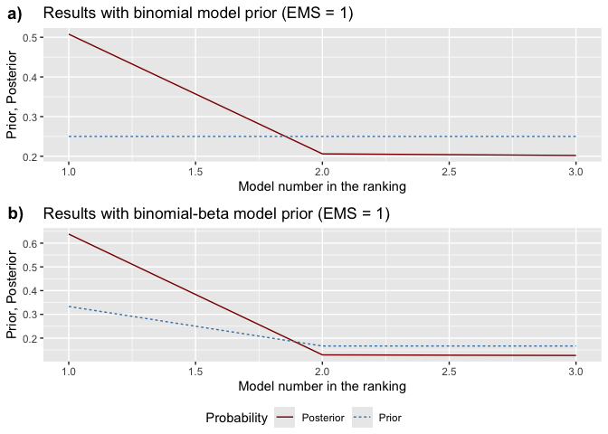


# Plot probabilities by model size
size_graphs <- bdsm::model_sizes(bma_results)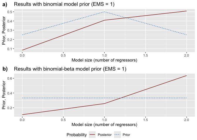

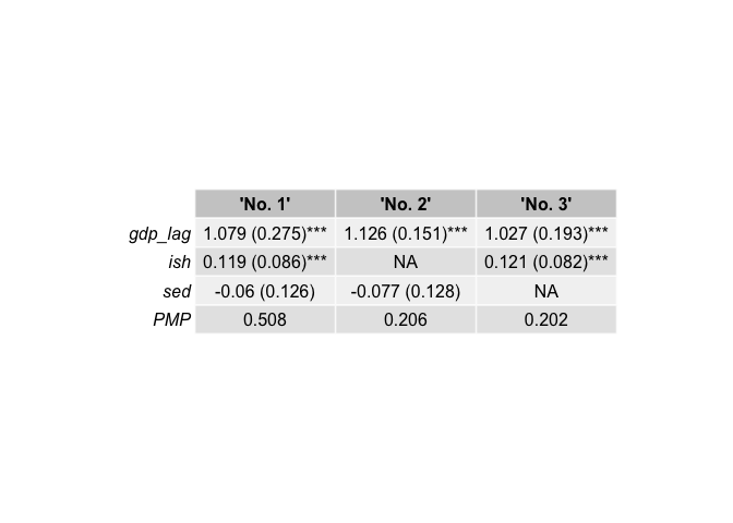
Selecting the Best Models

Use best_models() to extract specific information about the top-ranked models:

# Retrieve the 5 best models according to binomial prior
top3_binom <- bdsm::best_models(bma_results, criterion = 1, best = 3)


# Print the inclusion matrix for each of the top 3 models
top3_binom[[1]]
#>         'No. 1' 'No. 2' 'No. 3'
#> gdp_lag   1.000   1.000   1.000
#> ish       1.000   0.000   1.000
#> sed       1.000   1.000   0.000
#> PMP       0.508   0.206   0.202

# Retrieve robust standard errors in a knit-friendly table
top3_binom[[6]]

	‘No. 1’	‘No. 2’	‘No. 3’
gdp_lag	1.079 (0.275)***	1.126 (0.151)***	1.027 (0.193)***
ish	0.119 (0.086)***	NA	0.121 (0.082)***
sed	-0.06 (0.126)	-0.077 (0.128)	NA
PMP	0.508	0.206	0.202

Jointness Measures

Assess whether two regressors tend to co-occur (complements) or exclude each other (substitutes) using jointness(). By default, it calculates the Hofmarcher et al. (2018) measure:

joint_measures <- bdsm::jointness(bma_results)
head(joint_measures)
#>       ish   sed
#> ish    NA 0.159
#> sed 0.505    NA

You can also specify older measures, such as "LS" (Ley & Steel) or "DW" (Doppelhofer & Weeks):

joint_measures_ls <- bdsm::jointness(bma_results, measure = "LS")

Example

Below is a minimal reproducible workflow:

# 1) Data preparation
data_prepared <- bdsm::economic_growth[, 1:5] %>%
  bdsm::feature_standardization(
    excluded_cols = c(country, year, gdp)
  ) %>%
  bdsm::feature_standardization(
    group_by_col  = year,
    excluded_cols = country,
    scale         = FALSE
  )

# 2) Estimate model space
model_space <- bdsm::optim_model_space(
  df            = data_prepared,
  dep_var_col   = gdp,
  timestamp_col = year,
  entity_col    = country,
  init_value     = 0.5,
)
#> initial  value -427.743989 
#> final  value -717.595537 
#> converged
#> initial  value -366.799374 
#> final  value -784.520619 
#> converged
#> initial  value -396.225712 
#> final  value -785.991786 
#> converged
#> initial  value -238.285740 
#> final  value -854.671535 
#> converged

# 3) Run Bayesian Model Averaging
bma_obj <- bdsm::bma(
  model_space = model_space,
  df          = data_prepared
)

# 4) Inspect the top 3 models under binomial prior
best_3 <- bdsm::best_models(
  bma_list = bma_obj,
  criterion = 1,
  best = 3
)

best_3[[1]]  # Inclusion table
#>         'No. 1' 'No. 2' 'No. 3'
#> gdp_lag   1.000   1.000   1.000
#> ish       1.000   0.000   1.000
#> sed       1.000   1.000   0.000
#> PMP       0.508   0.206   0.202
best_3[[2]]  # Coefficients & standard errors
#>         'No. 1'            'No. 2'            'No. 3'           
#> gdp_lag "1.079 (0.111)***" "1.126 (0.106)***" "1.027 (0.093)***"
#> ish     "0.119 (0.033)***" NA                 "0.121 (0.03)***" 
#> sed     "-0.06 (0.063)"    "-0.077 (0.063)"   NA                
#> PMP     "0.508"            "0.206"            "0.202"

Troubleshooting

Cannot install required packages / setup renv environment

Make sure to go through the displayed errors. The problem might be connected to your OS environment. E.g. you might see an information like the following:

Configuration failed to find one of freetype2 libpng libtiff-4 libjpeg. Try installing:
 * deb: libfreetype6-dev libpng-dev libtiff5-dev libjpeg-dev (Debian, Ubuntu, etc)
 * rpm: freetype-devel libpng-devel libtiff-devel libjpeg-devel (Fedora, CentOS, RHEL)
 * csw: libfreetype_dev libpng16_dev libtiff_dev libjpeg_dev (Solaris)

In such case you should first try installing the recommended packages. With properly configured system environment everything should work fine.

References

Moral-Benito, E. (2016). “Model Averaging in Economics: An Overview.” Journal of Economic Surveys.
Ley, E. and Steel, M. F. J. (2007). “Jointness in Bayesian Variable Selection with Applications to Growth Regression.” Journal of Macroeconomics.
Doppelhofer, G. and Weeks, M. (2009). “Jointness of Growth Determinants.” Journal of Applied Econometrics.
Hofmarcher, P., Crespo Cuaresma, J., Huber, F., and Moser, M. (2018). “Forecasting with Bayesian Model Averaging: New Classical and Bayesian Perspectives.” Journal of Applied Econometrics.

(Additional references related to the methodology can be found in the package vignette.)

Contributions and Issues

We welcome bug reports, feature requests, and contributions. Feel free to open an issue or pull request on GitHub.

License

This package is distributed under the GPL (\(\geq 2\)) license. See the LICENSE file for details.