sdlrm:
Modified SDL Regression for Integer-Valued and Paired Count Data![]()
Rodrigo M. R. de Medeiros
Universidade Federal do Rio Grande do Norte, UFRN rodrigo.matheus@ufrn.br
Implementation of the modified SDL regression model proposed by
Medeiros and Bourguignon (2025). The sdlrm package provide
a set of functions for a complete analysis of integer-valued data, in
which it is assumed that the dependent variable follows a modified skew
discrete Laplace (SDL) distribution. This regression model is useful for
the analysis of integer-valued data and experimental studies in which
paired discrete observations are collected.
You can install the current development version of sdlrm
from GitHub with:
devtools::install_github("rdmatheus/sdlrm")To run the above command, it is necessary that the
devtools package is previously installed on R. If not,
install it using the following command:
install.packages("devtools")After installing the devtools package, if you are using Windows,
install the most current RTools
program. Finally, run the command
devtools::install_github("rdmatheus/sdlrm"), and then the
package will be installed on your computer.
This package provide complete estimation and inference for the
parameters as well as normal probability plots of residuals with a
simulated envelope, useful for assessing the goodness-of-fit of the
model. The implementation is straightforward and similar to other
popular packages, like betareg and glm, where
the main function is sdlrm(). Below is an example of some
functions usage and available methods.
# Loading the sdlrm package
library(sdlrm)

# Data visualization (Description: ?pss)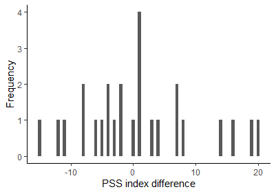
# Fit a double model (mean and dispersion)
fit0 <- sdlrm(difference ~ group | group, data = pss)

# Print
fit0
#>
#> Call:
#> sdlrm(formula = difference ~ group | group, data = pss)
#>
#> Mean Coefficients:
#> (Intercept)  groupSport
#>    7.363241  -11.296628
#>
#> Dispersion Coefficients:
#> (Intercept)  groupSport
#>   2.6555857  -0.5875779
#>
#> ---
#> Log-lik value: -88.56555
#> Mode: 0
#> AIC: 187.1311 and BIC: 193.4216

# Summary
summary(fit0)
#> Call:
#> sdlrm(formula = difference ~ group | group, data = pss)
#>
#>
#> Summary for quantile residuals:
#>       Mean Std. dev.  Skewness Kurtosis
#>   0.003877  0.948567 -0.096418 1.839793
#>
#>
#> Mean coefficients:
#>             Estimate Std. Error z value Pr(>|z|)
#> (Intercept)   7.3632     3.6010  2.0448 0.040874 *
#> groupSport  -11.2966     4.0119 -2.8158 0.004865 **
#> ---
#> Signif. codes:  0 '***' 0.001 '**' 0.01 '*' 0.05 '.' 0.1 ' ' 1
#>
#>
#> Dispersion coefficients with log link:
#>             Estimate Std. Error z value Pr(>|z|)
#> (Intercept)  2.65559    0.32089  8.2758   <2e-16 ***
#> groupSport  -0.58758    0.43006 -1.3663   0.1719
#> ---
#> Signif. codes:  0 '***' 0.001 '**' 0.01 '*' 0.05 '.' 0.1 ' ' 1
#>
#> ---
#> Log-lik value: -88.56555
#> Mode: 0
#> Pseudo-R2:0.1717017
#> AIC: 187.1311 and BIC: 193.4216
By default, the mode (\(\xi\)) of
the modified SDL distribution is fixed at \(\xi = 0\). It is possible to specify a
non-zero mode (it must be an integer value) using the xi
argument. Alternatively, this parameter can be estimated via profile
likelihood using the choose_mode() function:
## Mode estimation via profile likelihood
mode_estimation <- choose_mode(fit0)
#>
#> mode: -5 | logLik: -90.31 | AIC: 190.621 | BIC: 196.911
#> mode: -4 | logLik: -89.584 | AIC: 189.169 | BIC: 195.459
#> mode: -3 | logLik: -89.291 | AIC: 188.583 | BIC: 194.873
#> mode: -2 | logLik: -88.945 | AIC: 187.889 | BIC: 194.18
#> mode: -1 | logLik: -89.018 | AIC: 188.036 | BIC: 194.327
#> mode: 0 | logLik: -88.566 | AIC: 187.131 | BIC: 193.422
#> mode: 1 | logLik: -87.677 | AIC: 185.355 | BIC: 191.645
#> mode: 2 | logLik: -88.413 | AIC: 186.826 | BIC: 193.116
#> mode: 3 | logLik: -88.347 | AIC: 186.694 | BIC: 192.984
#> mode: 4 | logLik: -89.305 | AIC: 188.609 | BIC: 194.9
#> mode: 5 | logLik: -93.292 | AIC: 196.585 | BIC: 202.875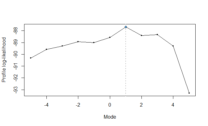
The mode_estimation object, of class
“choose_mode”, consists of a list whose elements represent
a modified SDL regression fit for each value specified for the mode (by
default, the sequence \(-5, -4, \ldots, 4,
5\)). We see that \(\xi = 1\)
generates the highest profiled likelihood.
## Double model with xi = 1
fit1 <- mode_estimation[[1]]
The constant dispersion test in the modified SDL regression can be
performed with the disp_test() function:
## Test for constant dispersion
disp_test(fit1)
#>            Score   Wald Lik. Ratio Gradient
#> Statistic 2.2968 2.2289     2.2625   2.2669
#> p-Value   0.1296 0.1354     0.1325   0.1322
The tests do not reject the null hypothesis of constant dispersion. We can then specify an adjustment with regressors only on the mean:
## Fit with constant dispersion and mode = 1
fit <- sdlrm(difference ~ group, data = pss, xi = 1)

## Summary
summary(fit)
#> Call:
#> sdlrm(formula = difference ~ group, data = pss, xi = 1)
#>
#>
#> Summary for quantile residuals:
#>       Mean Std. dev.  Skewness Kurtosis
#>   0.134617  0.982147 -0.282004 2.209202
#>
#>
#> Mean coefficients:
#>             Estimate Std. Error z value Pr(>|z|)
#> (Intercept)   5.6976     2.3592  2.4150 0.015733 *
#> groupSport  -11.3649     3.5272 -3.2221 0.001272 **
#> ---
#> Signif. codes:  0 '***' 0.001 '**' 0.01 '*' 0.05 '.' 0.1 ' ' 1
#>
#>
#> Dispersion coefficients with log link:
#>             Estimate Std. Error z value  Pr(>|z|)
#> (Intercept)  2.33085    0.21283  10.952 < 2.2e-16 ***
#> ---
#> Signif. codes:  0 '***' 0.001 '**' 0.01 '*' 0.05 '.' 0.1 ' ' 1
#>
#> ---
#> Log-lik value: -88.8298
#> Mode: 1
#> Pseudo-R2:0.3378125
#> AIC: 185.6596 and BIC: 190.692
Currently, the methods implemented for "sdlrm" objects
are
methods(class = "sdlrm")
#>  [1] AIC          coef         logLik       model.frame  model.matrix
#>  [6] plot         predict      print        residuals    summary
#> [11] vcov
#> see '?methods' for accessing help and source code
The plot() method provides diagnostic plots of the
residuals. By default, randomized quantile residuals are used:
par(mfrow = c(1, 2))
plot(fit, ask = FALSE)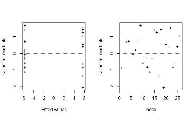
par(mfrow = c(1, 1))The envelope() function plots the normal probability of
the residuals with a simulated envelope:
## Building the envelope plot
envel <- envelope(fit, plot = FALSE)
#> | | | 0% | |= | 1% | |= | 2% | |== | 3% | |=== | 4% | |==== | 5% | |==== | 6% | |===== | 7% | |====== | 8% | |====== | 9% | |======= | 10% | |======== | 11% | |========= | 12% | |========= | 13% | |========== | 14% | |=========== | 15% | |=========== | 16% | |============ | 17% | |============= | 18% | |============== | 19% | |============== | 20% | |=============== | 21% | |================ | 22% | |================ | 23% | |================= | 24% | |================== | 26% | |=================== | 27% | |=================== | 28% | |==================== | 29% | |===================== | 30% | |===================== | 31% | |====================== | 32% | |======================= | 33% | |======================== | 34% | |======================== | 35% | |========================= | 36% | |========================== | 37% | |========================== | 38% | |=========================== | 39% | |============================ | 40% | |============================= | 41% | |============================= | 42% | |============================== | 43% | |=============================== | 44% | |=============================== | 45% | |================================ | 46% | |================================= | 47% | |================================== | 48% | |================================== | 49% | |=================================== | 50% | |==================================== | 51% | |==================================== | 52% | |===================================== | 53% | |====================================== | 54% | |======================================= | 55% | |======================================= | 56% | |======================================== | 57% | |========================================= | 58% | |========================================= | 59% | |========================================== | 60% | |=========================================== | 61% | |============================================ | 62% | |============================================ | 63% | |============================================= | 64% | |============================================== | 65% | |============================================== | 66% | |=============================================== | 67% | |================================================ | 68% | |================================================= | 69% | |================================================= | 70% | |================================================== | 71% | |=================================================== | 72% | |=================================================== | 73% | |==================================================== | 74% | |===================================================== | 76% | |====================================================== | 77% | |====================================================== | 78% | |======================================================= | 79% | |======================================================== | 80% | |======================================================== | 81% | |========================================================= | 82% | |========================================================== | 83% | |=========================================================== | 84% | |=========================================================== | 85% | |============================================================ | 86% | |============================================================= | 87% | |============================================================= | 88% | |============================================================== | 89% | |=============================================================== | 90% | |================================================================ | 91% | |================================================================ | 92% | |================================================================= | 93% | |================================================================== | 94% | |================================================================== | 95% | |=================================================================== | 96% | |==================================================================== | 97% | |===================================================================== | 98% | |===================================================================== | 99% | |======================================================================| 100%
par(mfrow = c(1, 2))
# Plot for the randomized quantile residuals (default)
plot(envel)
# Plot for the Pearson residuals
plot(envel, type = "pearson")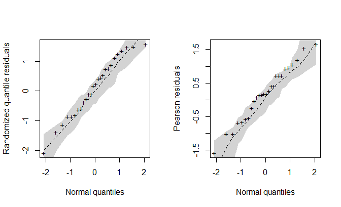
par(mfrow = c(1, 1))